Getting Started with VDJigsaw

Introduction

This vignette walks you through a typical VDJigsaw workflow using real-world VDJ data from 10x Genomics. By the end, you will have assigned clonotypes at multiple stringency levels and visualized the results.

What does VDJigsaw do? Single-cell TCR sequencing often suffers from dropout: a cell’s second alpha or beta chain allele may simply not get captured. Most tools treat missing chains as “different”, fragmenting clonotypes. VDJigsaw instead looks across the whole dataset to puzzle together which cells likely belong to the same clone, even when some chain data is missing. It does this at five levels of stringency, from strict (all four chains must match) to permissive (a single allele suffices).

Getting started

library(VDJigsaw)
library(dplyr)
library(ggplot2)
library(patchwork)

Load data

To illustrate VDJigsaw, we use VDJ filtered contig data from two publicly available 10x Genomics datasets:

10k Human Diseased PBMCs (ALL) — Freshly Processed (dataset | VDJ-TCR contigs)
10k Human Diseased PBMCs (ALL) — Fixed and Stored (dataset | VDJ-TCR contigs)

These CSV files are bundled with the package in inst/extdata/.

VDJ.contigs.fresh <- read.csv(system.file(
  "extdata",
  "10k_5p_Human_diseased_PBMC_ALL_Fresh_vdj_t_filtered_contig_annotations.csv",
  package = "VDJigsaw"))

VDJ.contigs.fix <- read.csv(system.file(
  "extdata",
  "10k_5p_Human_diseased_PBMC_ALL_Fix_stored_vdj_t_filtered_contig_annotations.csv",
  package = "VDJigsaw"))

For simplicity, we tag each dataset with a sample label and combine them:

VDJ.contigs.fresh$orig.ident <- "Fresh"
VDJ.contigs.fix$orig.ident   <- "Fix"
VDJ.contigs <- rbind(VDJ.contigs.fresh, VDJ.contigs.fix)

Let’s take a quick look at the raw data — each row is one contig (one chain from one cell):

cat(nrow(VDJ.contigs), "contigs across", length(unique(VDJ.contigs$barcode)), "unique barcodes\n")

## 27129 contigs across 13634 unique barcodes

knitr::kable(head(VDJ.contigs[, c("barcode", "chain", "v_gene", "cdr3", "j_gene", "umis", "orig.ident")], 5))

barcode	chain	v_gene	cdr3	j_gene	umis	orig.ident
AAACCAAAGAACAGAC-1	TRB	TRBV20-1	CSARDLYRGRETQYF	TRBJ2-5	25	Fresh
AAACCAAAGAACAGAC-1	TRA	TRAV8-4	CAVSDRQYSGGGADGLTF	TRAJ45	10	Fresh
AAACCAAAGAACAGAC-1	TRA	TRAV19	CALSGQTSGTYKYIF	TRAJ40	11	Fresh
AAACCAAAGCAAGATA-1	TRA	TRAV30	CGTYNSGNTGKLIF	TRAJ37	10	Fresh
AAACCAAAGCAAGATA-1	TRB	TRBV11-2	CASSLGRGRVAYEQFF	TRBJ2-1	7	Fresh

Run the pipeline

The main function assign_clonotype() runs the full VDJigsaw pipeline in four steps:

Pivot the long-format contigs into wide format (one row per cell, with TRA_1, TRA_2, TRB_1, TRB_2 columns)
Validate TCR chains (fix ordering, remove duplicates, flag invalid sequences)
Identify clonotypes at five stringency levels using graph-based clustering
Return annotated data and reference tables

You can set sample_col to tell VDJigsaw about your sample structure. The clone_loose parameter controls which stringency level becomes the default CloneID. Set num_cores to speed up processing when you have multiple samples (use -1 for all available cores).

Tip: Ideally, run VDJigsaw after quality control of your scRNA-seq data to remove low-quality barcodes and doublets, which could skew clonotype assignments.

VDJigsaw_res <- assign_clonotype(
  VDJ_data = VDJ.contigs,
  sample_col = "orig.ident",
  clone_loose = "single_chain_single_allele",
  num_cores = 1,
  verbose = TRUE)

## [VDJigsaw] ========================================

## [VDJigsaw] Starting VDJigsaw clonotype assignment

## [VDJigsaw] ========================================

## [VDJigsaw] Detected raw contig input — pivoting to wide format

## [VDJigsaw] Converting VDJ data to wide format...

## [VDJigsaw]   Using cdr3_nt for CDR3 chain identifier

## [VDJigsaw]   Pivoting to wide format...

## [VDJigsaw]   Wide format: 13639 unique barcodes

## [VDJigsaw]   Creating TRA/TRB chain columns...

## [VDJigsaw] Wide format conversion complete: 98 columns

## [VDJigsaw] Validating and correcting TCR data...

## [VDJigsaw] Removed 1 duplicate alleles (allele 1 == allele 2)

## [VDJigsaw] Swapped 8 alleles where allele_2 was defined but allele_1 was not

## [VDJigsaw] TCR data correction complete

## [VDJigsaw] Identifying clonotypes and building reference tables...

## [VDJigsaw] Checking inputs...

## [VDJigsaw] Processing 13639 cells across 2 sample(s)

## [VDJigsaw] Using 1 core(s) for parallel processing

## [VDJigsaw] Combining results from parallel processing...

## [VDJigsaw]   dual_chain_dual_allele: 7432 clonotypes identified

## [VDJigsaw]   dual_chain_one_partial: 7139 clonotypes identified

## [VDJigsaw]   dual_chain_both_partial: 7117 clonotypes identified

## [VDJigsaw]   single_chain_dual_allele: 7116 clonotypes identified

## [VDJigsaw]   single_chain_single_allele: 7116 clonotypes identified

## [VDJigsaw] Clonotype identification complete!

## [VDJigsaw] ========================================

## [VDJigsaw] Pipeline complete!

## [VDJigsaw] Assigned 13639 of 13639 cells (100%) to clonotypes

## [VDJigsaw] ========================================

The result is a list with two elements:

TCR_data — wide-format data frame (one row per cell) with TCR chains and clone IDs at every stringency level
ref_tables — named list of reference tables mapping each CloneID to its chain composition

Explore the outputs

TCR data

The TCR_data table has one row per cell barcode, with clone IDs at every stringency level:

TCR_data <- VDJigsaw_res$TCR_data
cat(nrow(TCR_data), "cells,", ncol(TCR_data), "columns\n")

## 13639 cells, 109 columns

Here are the clone ID columns — each cell gets an assignment at every stringency level:

clone_cols <- colnames(TCR_data)[grepl("^CloneID\\.", colnames(TCR_data))]
knitr::kable(head(TCR_data[, c("Sample", "barcode", clone_cols)], 6))

Sample	barcode	CloneID.dual_chain_dual_allele	CloneID.loose	CloneID.dual_chain_one_partial	CloneID.dual_chain_both_partial	CloneID.single_chain_dual_allele	CloneID.single_chain_single_allele
Fresh	AAACCAAAGAACAGAC-1	Clone_Fresh_1	Clone_Fresh_1	Clone_Fresh_1	Clone_Fresh_1	Clone_Fresh_1	Clone_Fresh_1
Fresh	AAACCAAAGCAAGATA-1	Clone_Fresh_2	Clone_Fresh_2	Clone_Fresh_2	Clone_Fresh_2	Clone_Fresh_2	Clone_Fresh_2
Fresh	AAACCAAAGCTGGTTA-1	Clone_Fresh_3	Clone_Fresh_3	Clone_Fresh_3	Clone_Fresh_3	Clone_Fresh_3	Clone_Fresh_3
Fresh	AAACCAGCACCTAACG-1	Clone_Fresh_4	Clone_Fresh_4	Clone_Fresh_4	Clone_Fresh_4	Clone_Fresh_4	Clone_Fresh_4
Fresh	AAACCAGCACGCGTTA-1	Clone_Fresh_5	Clone_Fresh_5	Clone_Fresh_5	Clone_Fresh_5	Clone_Fresh_5	Clone_Fresh_5
Fresh	AAACCAGCACTAGGAA-1	Clone_Fresh_6	Clone_Fresh_6	Clone_Fresh_6	Clone_Fresh_6	Clone_Fresh_6	Clone_Fresh_6

Reference tables

The ref_tables list contains one reference table per stringency level. Each table maps a CloneID to its TCR chain composition.

VDJigsaw_ref_tables <- VDJigsaw_res$ref_tables
names(VDJigsaw_ref_tables)

## [1] "dual_chain_dual_allele"     "dual_chain_one_partial"    
## [3] "dual_chain_both_partial"    "single_chain_dual_allele"  
## [5] "single_chain_single_allele" "loose"

Each reference table has columns for CloneID, Sample, and the TCR chains. Let’s define a small helper to display them compactly (showing only the V gene part of each chain to save space):

# Helper: show ref table with truncated chain names for readability
show_ref <- function(ref_tbl, n = 5) {
  display_cols <- intersect(c("CloneID", "Sample", "TRA_1", "TRA_2", "TRB_1", "TRB_2"), colnames(ref_tbl))
  df <- head(ref_tbl[, display_cols], n)
  # Shorten V_CDR3_J strings to just V gene for display
  for (col in intersect(c("TRA_1", "TRA_2", "TRB_1", "TRB_2"), colnames(df))) {
    df[[col]] <- ifelse(is.na(df[[col]]), NA, sub("_.*", "", df[[col]]))
  }
  knitr::kable(df, row.names = FALSE)
}

Stringency levels

The stringency levels are named along two axes: which chains are required (both alpha and beta, or just one) and how many alleles per chain (both alleles, or just one).

Level	Name	Chains required	Alleles per chain
1	`dual_chain_dual_allele`	Both alpha and beta	Both alleles (1 and 2)
2	`dual_chain_one_partial`	Both alpha and beta	One chain can have a single allele
3	`dual_chain_both_partial`	Both alpha and beta	Both chains can have a single allele
4	`single_chain_dual_allele`	alpha or beta alone	Both alleles (1 and 2)
5	`single_chain_single_allele`	alpha or beta alone	A single allele suffices

dual_chain_dual_allele

The strictest level. All four chain positions (TRA_1, TRA_2, TRB_1, TRB_2) must match exactly.

cat(nrow(VDJigsaw_ref_tables$dual_chain_dual_allele), "clonotypes\n")

## 7432 clonotypes

show_ref(VDJigsaw_ref_tables$dual_chain_dual_allele)

CloneID	Sample	TRA_1	TRA_2	TRB_1	TRB_2
Clone_Fresh_1	Fresh	TRAV19	TRAV8-4	TRBV20-1	NA
Clone_Fresh_10	Fresh	TRAV6	NA	TRBV20-1	NA
Clone_Fresh_100	Fresh	TRAV12-1	TRAV21	TRBV19	NA
Clone_Fresh_1000	Fresh	TRAV8-6	NA	TRBV28	NA
Clone_Fresh_1001	Fresh	TRAV8-6	NA	TRBV20-1	NA

dual_chain_one_partial

Both chains required, but one chain may have a missing secondary allele (no conflict allowed).

cat(nrow(VDJigsaw_ref_tables$dual_chain_one_partial), "clonotypes\n")

## 7139 clonotypes

show_ref(VDJigsaw_ref_tables$dual_chain_one_partial)

CloneID	Sample	TRA_1	TRA_2	TRB_1	TRB_2
Clone_Fresh_1	Fresh	TRAV19	TRAV8-4	TRBV20-1	NA
Clone_Fresh_10	Fresh	TRAV6	NA	TRBV20-1	NA
Clone_Fresh_100	Fresh	TRAV1-2	NA	TRBV6-5	NA
Clone_Fresh_1000	Fresh	TRAV19	NA	TRBV6-5	NA
Clone_Fresh_1001	Fresh	TRAV1-2	NA	TRBV20-1	NA

dual_chain_both_partial

Both chains required, but both may have a missing secondary allele.

cat(nrow(VDJigsaw_ref_tables$dual_chain_both_partial), "clonotypes\n")

## 7117 clonotypes

show_ref(VDJigsaw_ref_tables$dual_chain_both_partial)

CloneID	Sample	TRA_1	TRA_2	TRB_1	TRB_2
Clone_Fresh_1	Fresh	TRAV19	TRAV8-4	TRBV20-1	NA
Clone_Fresh_10	Fresh	TRAV6	NA	TRBV20-1	NA
Clone_Fresh_100	Fresh	TRAV1-2	NA	TRBV6-5	NA
Clone_Fresh_1000	Fresh	TRAV1-2	TRAV8-3	TRBV12-4	NA
Clone_Fresh_1001	Fresh	TRAV8-1	NA	TRBV5-1	NA

single_chain_dual_allele

Only one chain (alpha or beta) is required, but both alleles of that chain must match.

cat(nrow(VDJigsaw_ref_tables$single_chain_dual_allele), "clonotypes\n")

## 7116 clonotypes

show_ref(VDJigsaw_ref_tables$single_chain_dual_allele)

CloneID	Sample	TRA_1	TRA_2	TRB_1	TRB_2
Clone_Fresh_1	Fresh	TRAV19	TRAV8-4	TRBV20-1	NA
Clone_Fresh_10	Fresh	TRAV6	NA	TRBV20-1	NA
Clone_Fresh_100	Fresh	TRAV1-2	NA	TRBV6-5	NA
Clone_Fresh_1000	Fresh	TRAV1-2	TRAV8-3	TRBV12-4	NA
Clone_Fresh_1001	Fresh	TRAV8-1	NA	TRBV5-1	NA

single_chain_single_allele

The most permissive level. A single allele of a single chain can define a clonotype. Maximizes cell recovery but should be used with caution.

cat(nrow(VDJigsaw_ref_tables$single_chain_single_allele), "clonotypes\n")

## 7116 clonotypes

show_ref(VDJigsaw_ref_tables$single_chain_single_allele)

CloneID	Sample	TRA_1	TRA_2	TRB_1	TRB_2
Clone_Fresh_1	Fresh	TRAV19	TRAV8-4	TRBV20-1	NA
Clone_Fresh_10	Fresh	TRAV2	NA	TRBV14	NA
Clone_Fresh_100	Fresh	TRAV26-1	NA	NA	NA
Clone_Fresh_1000	Fresh	TRAV21	NA	TRBV6-5	NA
Clone_Fresh_1001	Fresh	TRAV26-2	NA	TRBV5-4	NA

Let’s see how the number of clonotypes changes across levels:

sapply(VDJigsaw_ref_tables[1:5], nrow)

##     dual_chain_dual_allele     dual_chain_one_partial 
##                       7432                       7139 
##    dual_chain_both_partial   single_chain_dual_allele 
##                       7117                       7116 
## single_chain_single_allele 
##                       7116

As expected, the number of unique clonotypes decreases as stringency is relaxed (cells get merged into larger groups).

Visualize results

VDJigsaw includes three built-in visualization functions. All support per_sample and combined arguments for multi-sample datasets.

Stringency summary

This two-panel chart shows (top) the number of unique clonotypes and (bottom) the number of cells assigned at each stringency level.

plot_stringency_summary(
  TCR_data = TCR_data,
  per_sample = TRUE,
  combined = TRUE)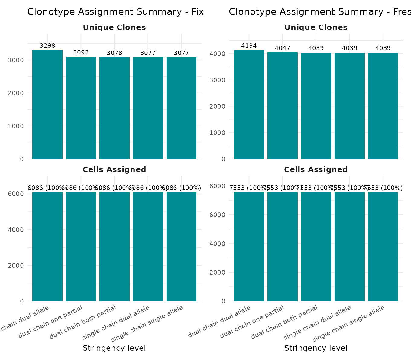

Clonotype composition

A tile chart showing V gene usage for the top clonotypes at a given stringency level. Grey tiles indicate missing chains.

Strict definition

plot_list <- plot_clone_composition(
  ref_table = VDJigsaw_ref_tables$dual_chain_dual_allele,
  top_n = 10,
  per_sample = TRUE,
  combined = FALSE)

plot_list$Fix +
  plot_list$Fresh +
  plot_layout(ncol = 1)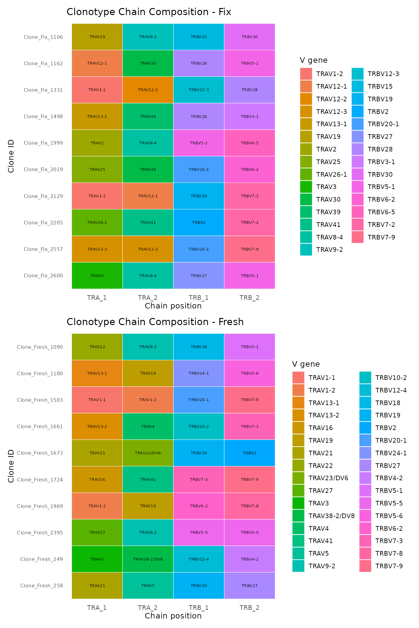

Loose definition

plot_list <- plot_clone_composition(
  ref_table = VDJigsaw_ref_tables$single_chain_single_allele,
  top_n = 10,
  per_sample = TRUE,
  combined = FALSE)

plot_list$Fix +
  plot_list$Fresh +
  plot_layout(ncol = 1)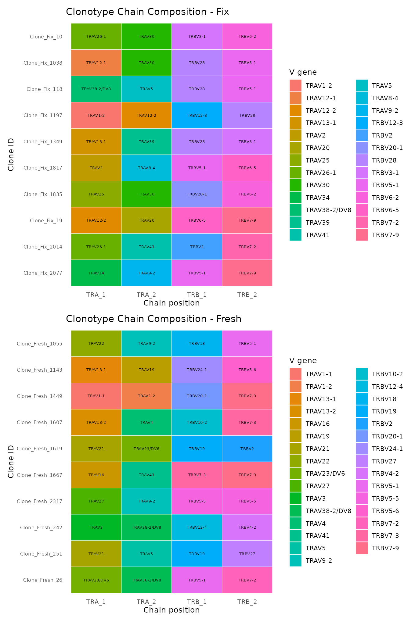

Clonotype flow (alluvial)

An alluvial diagram showing how clonotypes merge as stringency is relaxed. Each vertical axis is a stringency level, and flows show cells moving between clone definitions.

plot_list <- plot_clonotype_flow(
  TCR_data = TCR_data,
  top_n = 10,
  per_sample = TRUE,
  combined = FALSE)

plot_list$Fix +
  plot_list$Fresh +
  plot_layout(ncol = 1)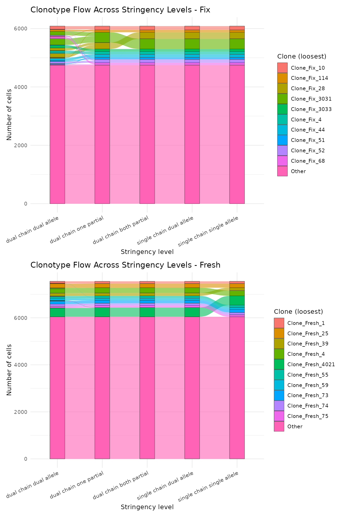

Next steps

Integrate with Seurat: Map TCR_data back to your Seurat object using the barcode column to annotate cells with clone IDs.
Cross-reference: Use assign_clonotype_from_reference() to map new data against an existing reference clonotype table.
Paired TCR mapping: Use map_clonotypes_to_paired_TCR() to match allele-level data to a paired alpha/beta reference.

For more details, see the function documentation: ?assign_clonotype, ?assign_clonotype_from_reference, ?map_clonotypes_to_paired_TCR.

Session Info

sessionInfo()

## R version 4.5.2 (2025-10-31)
## Platform: x86_64-pc-linux-gnu
## Running under: Ubuntu 24.04.3 LTS
## 
## Matrix products: default
## BLAS:   /usr/lib/x86_64-linux-gnu/openblas-pthread/libblas.so.3 
## LAPACK: /usr/lib/x86_64-linux-gnu/openblas-pthread/libopenblasp-r0.3.26.so;  LAPACK version 3.12.0
## 
## locale:
##  [1] LC_CTYPE=C.UTF-8       LC_NUMERIC=C           LC_TIME=C.UTF-8       
##  [4] LC_COLLATE=C.UTF-8     LC_MONETARY=C.UTF-8    LC_MESSAGES=C.UTF-8   
##  [7] LC_PAPER=C.UTF-8       LC_NAME=C              LC_ADDRESS=C          
## [10] LC_TELEPHONE=C         LC_MEASUREMENT=C.UTF-8 LC_IDENTIFICATION=C   
## 
## time zone: UTC
## tzcode source: system (glibc)
## 
## attached base packages:
## [1] stats     graphics  grDevices utils     datasets  methods   base     
## 
## other attached packages:
## [1] patchwork_1.3.2 ggplot2_4.0.2   dplyr_1.2.0     VDJigsaw_0.1.0 
## 
## loaded via a namespace (and not attached):
##  [1] sass_0.4.10        generics_0.1.4     tidyr_1.3.2        stringi_1.8.7     
##  [5] digest_0.6.39      magrittr_2.0.4     evaluate_1.0.5     grid_4.5.2        
##  [9] RColorBrewer_1.1-3 iterators_1.0.14   fastmap_1.2.0      foreach_1.5.2     
## [13] doParallel_1.0.17  jsonlite_2.0.0     purrr_1.2.1        scales_1.4.0      
## [17] codetools_0.2-20   textshaping_1.0.4  jquerylib_0.1.4    cli_3.6.5         
## [21] rlang_1.1.7        withr_3.0.2        cachem_1.1.0       yaml_2.3.12       
## [25] tools_4.5.2        parallel_4.5.2     vctrs_0.7.1        R6_2.6.1          
## [29] lifecycle_1.0.5    stringr_1.6.0      fs_1.6.6           ragg_1.5.0        
## [33] pkgconfig_2.0.3    desc_1.4.3         pkgdown_2.2.0      pillar_1.11.1     
## [37] bslib_0.10.0       gtable_0.3.6       glue_1.8.0         systemfonts_1.3.1 
## [41] xfun_0.56          tibble_3.3.1       tidyselect_1.2.1   knitr_1.51        
## [45] farver_2.1.2       htmltools_0.5.9    igraph_2.2.2       rmarkdown_2.30    
## [49] labeling_0.4.3     ggalluvial_0.12.5  compiler_4.5.2     S7_0.2.1

Rémy Pétremand

17 February, 2026